Understanding LLM Inference Engines: Inside Nano-vLLM (Part 2)

Model Internals, KV Cache, and Tensor Parallelism

In Part 1, we explored the engineering architecture of Nano-vLLM: how requests flow through the system, how the Scheduler batches sequences, and how the Block Manager tracks KV cache allocations. We deliberately treated the model computation as a black box. Now it’s time to open that box.

This part dives into the model itself: how tokens become vectors, what happens inside each decoder layer, how KV cache is physically stored on GPU memory, and how tensor parallelism splits computation across multiple GPUs. By the end, you’ll have a complete picture of what happens from the moment a prompt enters the system to when generated text comes out.

What Is a Model, Really?

When we talk about “a model,” we often think of the weights—those massive files measured in billions of parameters. But a model that can actually run inference requires three components:

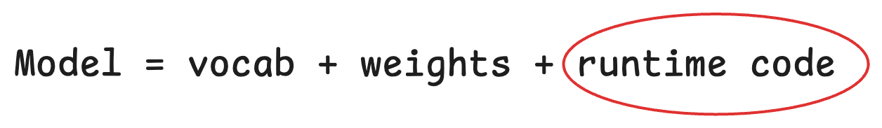
• Vocabulary: A static mapping between tokens and their IDs. This is how the model translates between human-readable text and the numerical representations it actually processes.
• Weights: The learned parameters—the “knowledge” accumulated during training. A 7B model has 7 billion of these parameters.
• Runtime Code: The logic that defines how to use the weights to transform inputs into outputs. This is the part that actually executes on GPUs.

Why Inference Engines Implement Model Code

You might wonder: if model providers release weights, why don’t they also release the runtime code? Many do—but there’s a catch. Runtime code must be optimized for specific scenarios: training vs. inference, different GPU architectures, different precision formats. What works for training on a cluster of A100s may not be optimal for inference on a single consumer GPU.

This is why inference engines like vLLM implement their own model code. The full vLLM repository contains optimized implementations for dozens of model architectures—Qwen, LLaMA, DeepSeek, Mistral, and more. Nano-vLLM simplifies this by supporting only Qwen, but the patterns are universal.

The Model Pipeline

Let’s trace what happens to a token as it flows through the model.

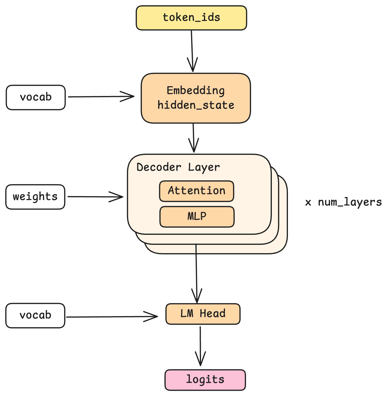
Embedding: Tokens to Vectors

The journey begins with embedding. A token ID is just a number—say, 1547. The embedding layer looks up this ID in the vocabulary and retrieves a vector: a high-dimensional array of floating-point numbers (4096 dimensions in the Qwen model Nano-vLLM uses). This vector, called a hidden state, is the model’s internal representation of that token.

Why 4096 dimensions? This is a design choice that balances expressiveness against computational cost. More dimensions can capture more nuanced meanings, but require more computation and memory.

Decode Layers: Where the Magic Happens

The hidden state then passes through a stack of decode layers—24 of them in the Qwen model that Nano-vLLM supports. Each layer performs the same operations but with different learned weights, progressively refining the representation. You can think of each layer as adding another layer of understanding: perhaps one layer captures syntactic relationships, another captures semantic meaning, another handles factual knowledge. (In reality, what each layer learns is emergent from training, not explicitly designed.)

The key property: each layer takes a hidden state as input and produces a hidden state as output, both with the same shape (4096 dimensions). This uniformity is what allows layers to be stacked.

LM Head: Vectors Back to Tokens

After all decode layers, the final hidden state is transformed back into a probability distribution over the vocabulary. This is the job of the LM head (language model head), which essentially reverses the embedding process. The output is logits—a score for every possible next token, which sampling then converts into an actual token selection.

Inside a Decode Layer

Each decode layer contains two main stages: Attention and MLP. Let’s examine each.

Multi-Head Attention

Attention is the mechanism that allows each token to “look at” other tokens in the sequence. But modern LLMs don’t use simple attention—they use multi-head attention, which splits the attention computation into multiple parallel “heads.”

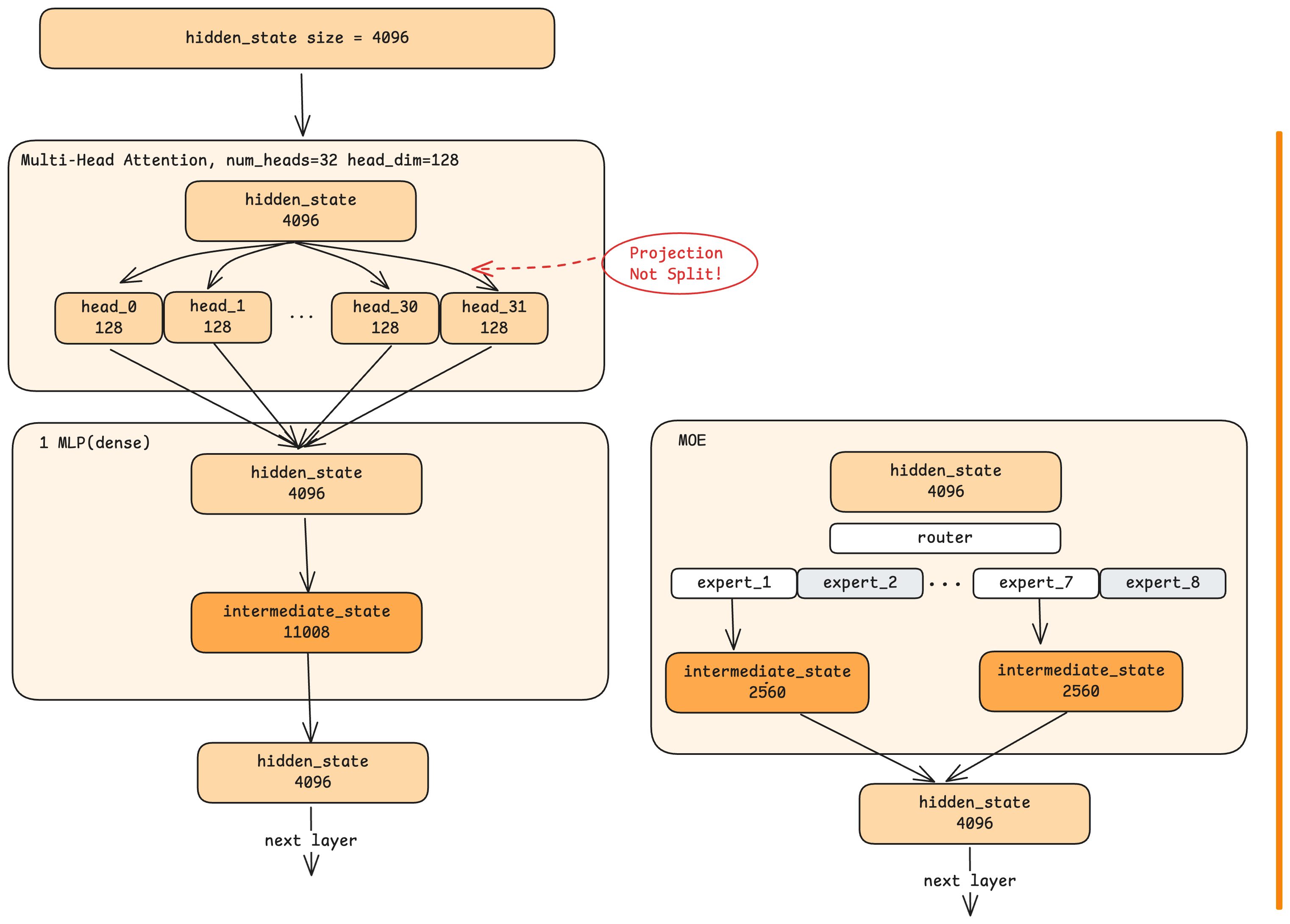
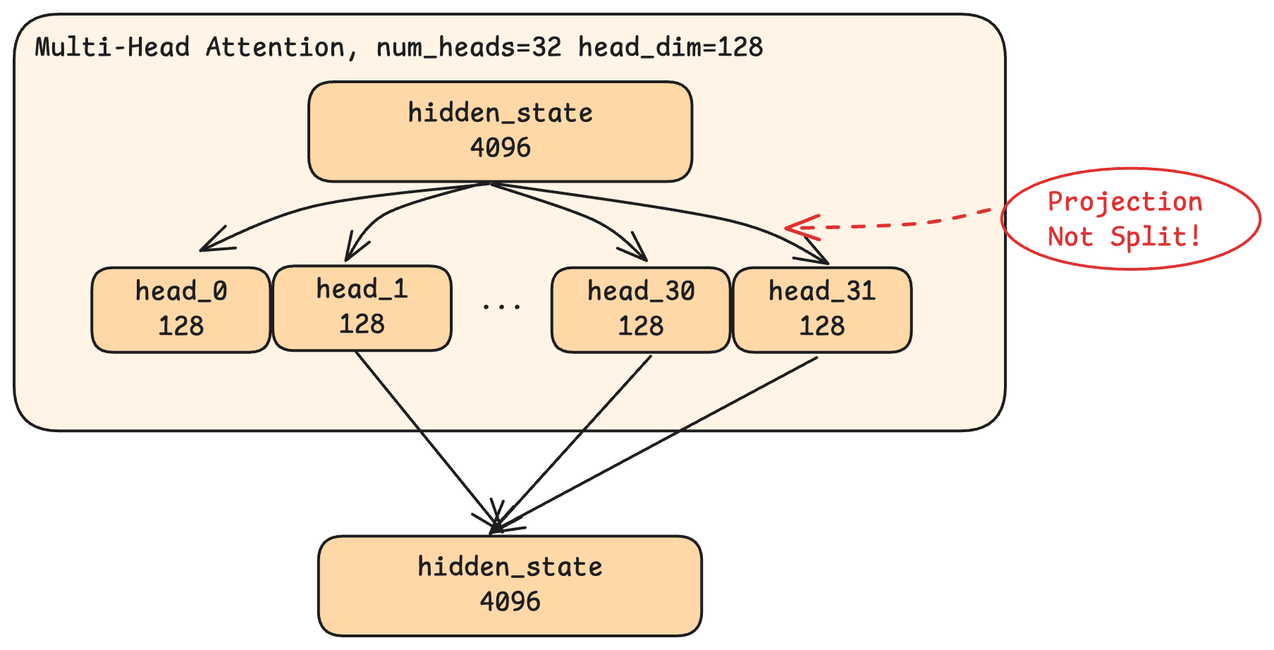
In the Qwen model, there are 32 heads, each working with 128-dimensional slices (32 × 128 = 4096, the full hidden state size). Here’s the crucial insight: this is not simply dividing the 4096 dimensions into 32 groups. Instead, each head performs a projection—a learned transformation that compresses the full 4096-dimensional input into a 128-dimensional representation specific to that head.

Think of it like a factory with 32 specialized workstations on the assembly line. Each workstation receives the same raw material (the full 4096-dimensional input) but uses different tooling to shape it in a particular way. One workstation might cut for grammatical fit, another might polish for semantic coherence, another might measure positional alignment—though in practice, what each workstation learns to do is also emergent and not so cleanly interpretable.

Each head also participates in the “attention” mechanism proper: it computes how much the current token should attend to each previous token in the sequence. This is where the model captures context—understanding that it in “The cat sat on the mat. It was comfortable.” refers to “the cat.”

After all heads complete their computations, their outputs are concatenated and projected back to 4096 dimensions, producing the layer’s attention output.

MLP: Self-Refinement

The MLP (Multi-Layer Perceptron) stage takes the attention output and refines it further. Unlike attention, MLP doesn’t look at other tokens—it processes each token’s hidden state independently.

The MLP first expands the hidden state from 4096 to a larger intermediate dimension (11008 in Qwen), applies a non-linear activation function, then compresses back to 4096. Why this expansion and compression?

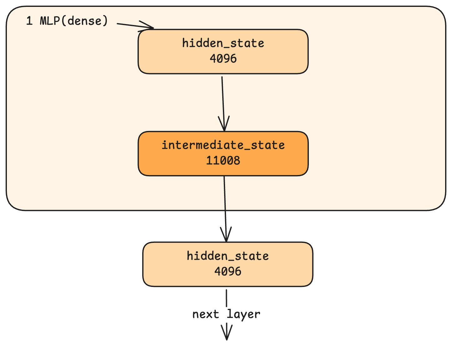
Think of it as enhancing resolution. The 4096-dimensional hidden state is like a compressed image. Expanding to 11008 dimensions is like upscaling—it creates room to add detail, informed by the MLP’s learned weights. The compression back to 4096 then distills this enriched representation. Through this process, the model incorporates knowledge from its training into each token’s representation.

Dense vs. MoE Architectures

The MLP we just described is a dense architecture: every token passes through the same single MLP block. But some modern models use Mixture of Experts (MoE), which takes a different approach.

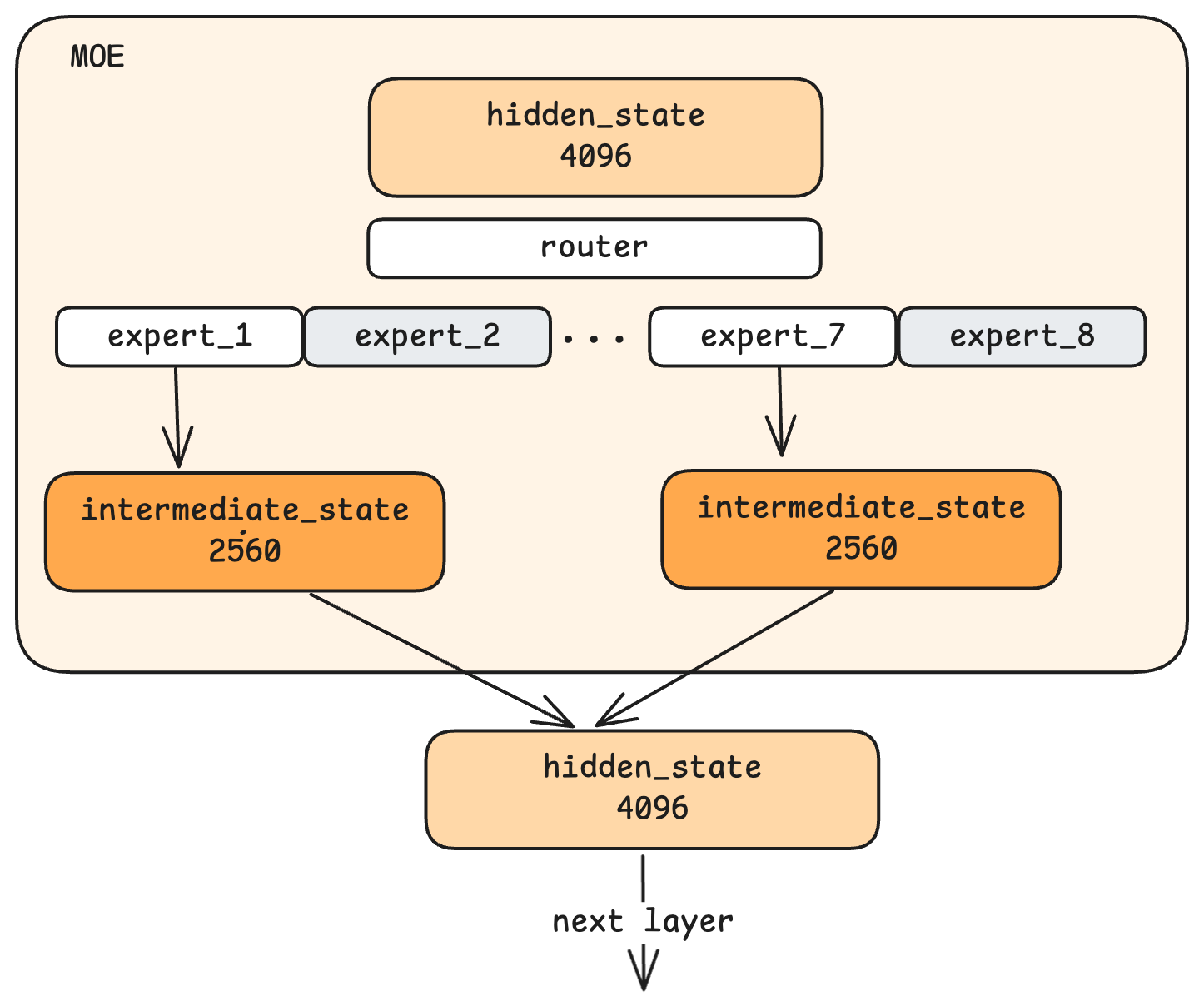
In MoE, instead of one large MLP, there are multiple smaller “expert” MLPs—say, 8 of them. A router network examines each incoming hidden state and decides which experts should process it. For example, only 2 out of 8 experts are activated for any given token.

The term “expert” might suggest human-interpretable specialization—one expert for math, another for language, another for coding. In practice, what each expert learns is emergent from training, not explicitly designed. We can’t easily characterize what makes Expert 3 different from Expert 5.

So why use MoE? The primary motivation is computational efficiency, not output quality. With MoE, you can have a model with a large total parameter count (all experts combined) while only activating a fraction of those parameters for each token. This dramatically reduces computation per token.

The trade-off: given the same total parameter count, a dense model will generally produce higher-quality outputs than an MoE model, because the dense model uses all its parameters for every token. But dense models at very large scales become computationally prohibitive to train. MoE allows scaling to parameter counts that would be infeasible with dense architectures—accepting somewhat lower per-parameter efficiency in exchange for practical trainability.

KV Cache: The Data Plane

In Part 1, we discussed the Block Manager as the control plane for KV cache—tracking allocations in CPU memory. Now let’s examine the data plane: how KV cache is actually stored on GPU memory.

What Gets Cached

During attention computation, each token produces two vectors: K (key) and V (value). These are used to compute attention scores with subsequent tokens. Rather than recomputing K and V for all previous tokens at every decode step, we cache them.

The Physical Layout

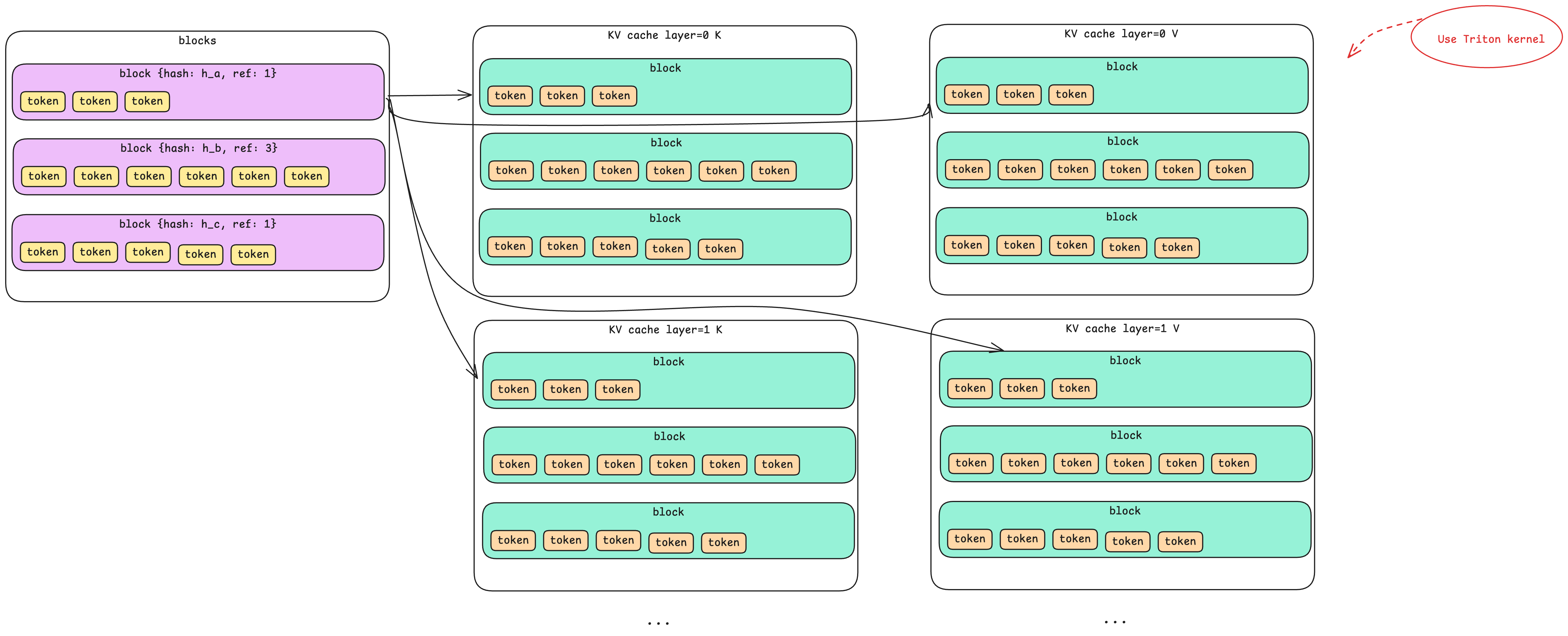
The KV cache on GPU is organized as a multi-dimensional structure:

• Block dimension: Matching the Block Manager’s logical blocks (e.g., 256 tokens per block)
• Layer dimension: Each of the 24 decode layers has its own cache, because attention is computed independently at each layer
• K/V dimension: Two separate caches per layer—one for keys, one for values
• Token dimension: Within each block, space for each token’s cached vectors

So a single logical block in the Block Manager corresponds to 24 × 2 = 48 physical cache regions on GPU—one K cache and one V cache for each of the 24 layers.

Triton Kernels for Cache Access

Nano-vLLM doesn’t manipulate GPU memory directly through CUDA APIs. Instead, it uses Triton kernels—high-level GPU programs that compile to efficient CUDA code. These kernels handle reading from and writing to the KV cache, abstracting away the complexity of GPU memory management.

Tensor Parallelism: Computation Level

In Part 1, we covered tensor parallelism’s communication pattern—how the leader broadcasts commands via shared memory. Now let’s see how the actual computation is split across GPUs.

Parallelism in Attention

Consider TP=2 (two GPUs). When a hidden state enters the attention stage:

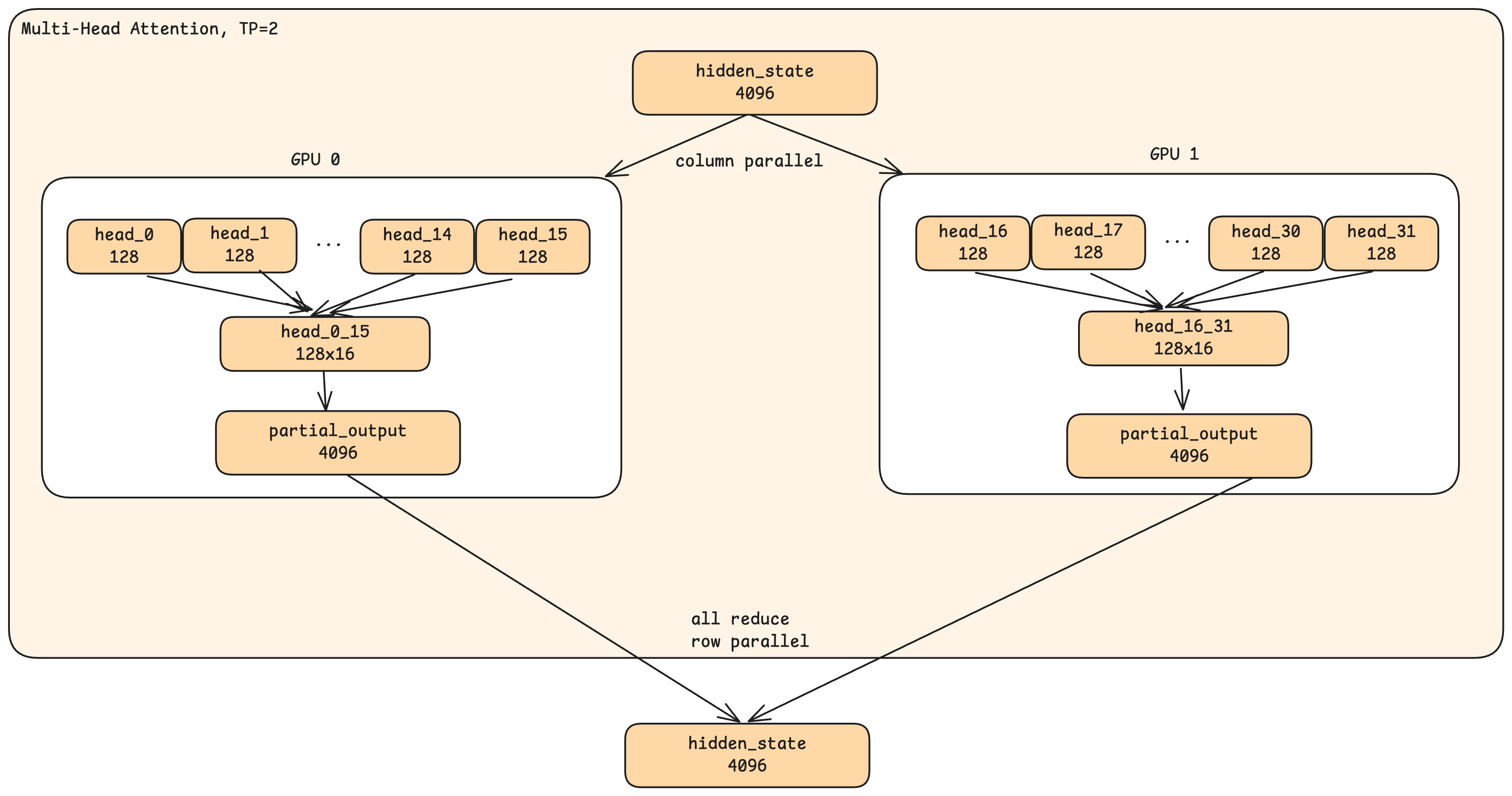
1. Both GPUs receive the complete hidden state (4096 dimensions). This is not a split—each GPU has the full input.
2. Each GPU handles half the heads. GPU 0 processes heads 0-15; GPU 1 processes heads 16-31.
3. Each GPU produces a partial output. GPU 0’s output incorporates only heads 0-15; GPU 1’s output incorporates only heads 16-31.
4. All-reduce combines the results. The GPUs exchange their partial outputs and sum them, so both end up with the complete attention output.

The key insight: parallelism happens in the head dimension, not the hidden state dimension. Each GPU sees the full input but computes only its assigned heads.

Parallelism in MLP

MLP parallelism follows a similar pattern:

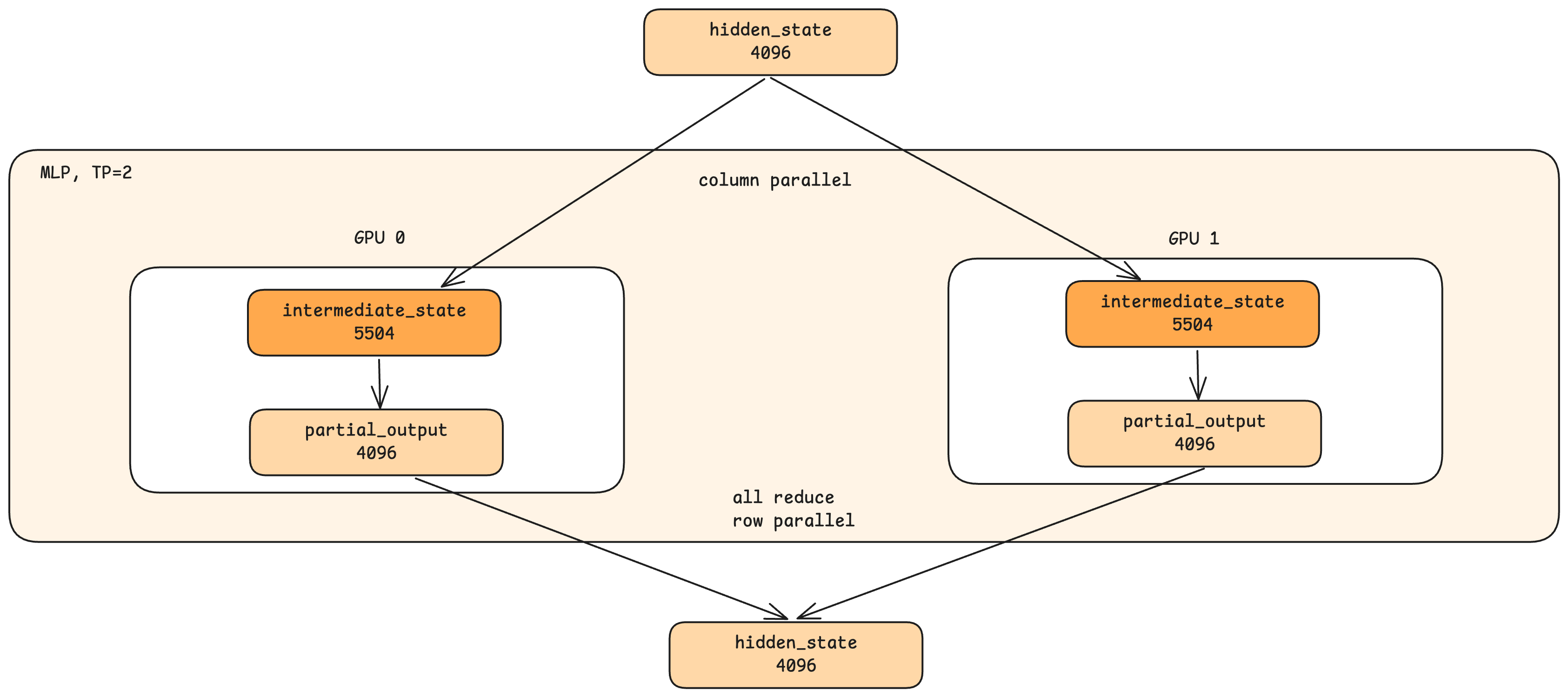
1. Both GPUs receive the complete hidden state.
2. The intermediate dimension is split. If the full MLP expands to 11008 dimensions, each GPU computes 5504 dimensions.
3. Each GPU produces a partial output.
4. All-reduce combines the results.

The Cost of Communication

Tensor parallelism isn’t free. The all-reduce operations require GPU-to-GPU communication, which adds latency. This is why TP is most effective on single-machine multi-GPU setups with fast interconnects (like NVLink), rather than across network-connected machines where communication latency would dominate.

The benefit: each GPU needs to store only a fraction of the model weights (half for TP=2, one-eighth for TP=8). This allows running models that wouldn’t fit on a single GPU’s memory.

Reflections: Design Trade-offs

Having seen the internals, let’s consider some design questions that often arise.

What Do Layers and Heads Control?

More layers generally enable deeper reasoning—each layer adds another pass of refinement over the hidden state. More heads enable richer attention patterns—more “perspectives” for understanding token relationships.

Can we create a narrow-but-deep model (few heads, many layers) for specialized deep reasoning? Or a wide-but-shallow model (many heads, few layers) for broad knowledge? Research suggests this doesn’t work well. Like human learning, models seem to benefit from a balance of breadth and depth. Extremely unbalanced architectures tend to underperform. Most successful models maintain a roughly square-ish ratio between these dimensions.

The practical levers for model capability remain the training data (what knowledge is available) and training methodology (how effectively that knowledge is learned), rather than architectural extremes.

Why Is MoE Becoming Popular?

MoE’s rise isn’t because it produces better outputs per parameter—it doesn’t. A 70B dense model will generally outperform a 70B MoE model (where 70B is the total across all experts).

MoE is popular because it enables scale. Training a 600B dense model is computationally prohibitive with current infrastructure. But a 600B MoE model that activates only 50B parameters per token? That’s trainable—and despite the per-parameter efficiency loss, the sheer scale can achieve capabilities that no trainable dense model could match.

This is a pragmatic engineering trade-off: accept lower efficiency per parameter in exchange for reaching scales that would otherwise be impossible.

Conclusion

We’ve now traced the complete journey from prompt to generated text:

1. Tokenization converts text to token IDs
2. Embedding converts token IDs to hidden state vectors
3. Decode layers refine hidden states through attention (cross-token understanding) and MLP (knowledge integration)
4. KV cache stores intermediate attention results to avoid redundant computation
5. LM head converts final hidden states to token probabilities
6. Sampling selects output tokens from probability distributions
7. Tensor parallelism enables all of this to scale across multiple GPUs

The inference engine orchestrates this entire pipeline—scheduling requests, managing memory, coordinating parallel execution—while the model architecture defines the computation within each step.

Understanding these internals demystifies what can seem like magic. An LLM is, at its core, a sophisticated function: vectors in, vectors out. The intelligence emerges from the scale of parameters, the quality of training data, and the clever engineering that makes it all run efficiently.

Whether you’re deploying models in production, debugging performance issues, or simply curious about how these systems work, this foundation should serve you well.